Alan Montgomery
218 Mccurdy DR.
Kanata, ON K2L 2L6
Canada

KEYWORDS: Velocity of light, Regression Model, Sensitivity, Young earth model.

INTRODUCTION

In 1987 Setterfield published his monograph Atomic Constants, Light and Time[19] which raised again the question of the constancy of c. Since then there have been no less than 17 articles in the Creation Research Society Quarterly and 12 articles in the Creation Ex Nihilo Technical Journal debating this issue. Authors have used various statistical techniques including run tests, regression lines, weighted regression lines and distribution tests. One important claim made by Setterfield is that the decreasing c hypothesis explains how the transit time of light from galaxies billions of light years away takes only thousands of years. Since it would provide an alternative to well accepted scientific arguments against the credibility of biblical history and chronologies this hypothesis should be welcome among young-earth creationists. However, this has not been the case. Since this hypothesis is potentially very significant to creationist astronomy and physics, it is important to develop data and tests which are unambiguous. This paper defines a data set of c values appropriate to this purpose and analyzes this data not only for trends but also for non-physical explanations of the trends in the data.

One of the primary motivations for this analysis of the data on the velocity of light stems from a dissatisfaction with the techniques and data used in previous analyses, including my own [16]. Most analyses have used 162 or 163 data from Setterfield's tables as their basic data. If these had provided unambiguous results the matter would be settled. However, some of Setterfield's data is either non-experimental (Encyclopedia Britannica 1771), duplicate (Cornu 1874) or regarded as unreliable (Young/Forbes 1881). This gives undue weight to some experiments and undermines the credibility of the results. Previous studies have also ignored the question of the sensitivity of the data and methods i.e., the ability of the data to detect a change of the size suggested by Setterfield. Thus, some data, which lack precise or accuracy, render the data collectively ambiguous. This study incorporates the principle of one datum to each experiment and the use of data only if it is sufficiently precise and consistent to distinguish between a constant and a decrease of the size claimed by Setterfield.

METHOD OF DATA SELECTION

Data has been drawn from four secondary sources: Setterfield [19], Froome and Essen [11], Dorsey [7] and Birge [2]. As there is agreement in these sources concerning the original published values no search of the original sources was made. The values from these four sources have been collected into a single table of 207 values (Appendix A). From these I removed duplicate values and constructed a second table of single valued independent experimental data (SVIED) which contains 158 values, one single value for every recognized experiment (S and D's removed from Appendix A). The SVIED was then analyzed for methods or data which were not acceptable because they were outliers, rejected by scientific authorities or contained anomalous and unacceptable characteristics. The remaining 119 values (SVIEAD) were subjected to a sensitivity analysis. Three additional data were eliminated by the sensitivity analysis leaving 116 data accepted for analysis (DAFA; * or M* in Appendix A). The error bars were taken from the secondary sources except for Setterfield's data where the error bars quoted in Hasofer's regression analysis [13] were used. One exception to this is the error bar for Delambre which is decidedly too small and was increased to a more modest 1000 km/sec. For data which appeared in more than one source the errors were the same with two or three exceptions. The primary use of this data was in justifying the variance assumption of the weighted regression technique and secondarily in the analysis by error bar size.

Single Valued Independent Experimental Data

The data in Appendix A contains many multiple values. These may be divided into three categories. First, there are the values which have been recalculated to take into account some factor missing from the originally published value. Such original values are labeled D as defective. Mostly, these are in vacuo corrections. The second group contains values which were computed from the same original observations but with different statistical treatment. These are reworkings and are labeled M* as multiple values. These have been reduced to single values by taking the median of the various reworkings. The third category are data which were rejected by the experimenters, for example Cornu (1872), and replaced by a subsequent value from a new experiment. Typically, these new data have improved accuracy and precision. These have also been labeled D. Omitted are values which are averages of other data, including the 1771 Encyclopedia Britannica value, and values quoted from unidentified sources. These have been labeled S for secondary. In addition to removing duplicates, values were added which had previously been lumped into a single average but were experimentally different. The early aberration values from Bradley's research contains observations of different stars at 3 different observatories at different times and deserve to be recognized as separate data points. These values were calculated from Table 2 of Setterfield and Norman. [191]

Unacceptable Methods And Rejected Data

Four methods contain data the majority of which is questionable: radar, quartz modulator, EMU/ESU and Kerr cell. Three radar values are in air and have not been converted to in vacuo for lack of humidity measurements. Radar waves are more sensitive to humidity than visible light so that the usual factor of 1.0002885 may be low [11, p79]. The possible range of the conversion factor is sufficient to cause the radar values to be ambiguous with respect to the hypothesis. Froome and Essen also consider these to be of poor accuracy [11, p79] and, since no humidity measurements were taken, unsuitable for conversion to in vacuo. These have been omitted. The large error bars (in comparison with the other post 1945 data) suggests they would be of little value. The quartz modulator values were considered poor by Froome and Essen. They quote Houstoun: "to say that its (minimum intensity) determination gives no feeling of aesthetic satisfaction is an understatement" [11, p84]. Neither value would survive an outlier analysis and so have been omitted. The EMU/ESU method contains 10 values from 1868 to 1883 which by simple regression line yield an anomalous 934+185 km/sec/year increase. This is clearly an experimental problem not related to any physical changes in the value of c. The magnitude of this change and the number of data is sufficient to produce a rate of increase over 188+85 km/sec/yr for the data as a whole. Exactly where this anomaly ends is difficult to tell and it must be admitted that the decision of Birge, Dorsey and Setterfield to omit all but the Dorsey 1906 datum is a necessary one. The values of the Kerr cell method are unquestionably low in comparison to post 1945 data [17]. However, no reviewer to my knowledge has been able to find errors of the size which would reconcile these results. This method was included since Birge, Dorsey and Setterfield included them in their best data.

Rejects are data whose values have been questioned by authorities because of experimental limitations or me lack of credible result. These have been labeled RJR in the Appendix A. Todd [21] in his article on solar parallax excluded both the Fizeau (1849) and Foucault (1862) values from his weighted average of c. DeBray [6] listed all the optical values prior to 1931 and selected only seven which he considered trustworthy. Fizeau (1849), Foucault (1862), Michelson (1878), Young/Forbes (1880), Newcomb (1881.8) and Cornu (1872) were among the values described as preliminary or flawed by systematic errors. Among the optical data I differ from DeBray only in the use of the first and second value of the Perrotin/Prim (1900) experiments, while DeBray treats them as a single experiment. Mulligan and McDonald [17] comment extensively on the Spectral line method. Concerning the 1952 value they comment that Rank later found a systematic error which increased the total error to 15 km/sec. The Rank (1954) value was flawed by a poor wavelength which obviously affected the prior value as well. The aforementioned values are treated either as 'rejecteds or as defective preliminary values replaced later by a superior datum.

An adjustment for aberration values is necessary before the data is prepared for analysis. The aberration values are calculated from the aberration angle of starlight in air. These calculated values are, thus, in air rather than in vacuo values. Since none of the sources has calculated these individually or suggested an adjustment collectively I added 95 km/sec [11, p48] to each the datum.

Outliers

For the outlier analysis data was divided into three sections: the early data up to 1890, the middle data from 1890 to 1940 and the late data from 1947 to 1967. Data were considered to be outliers if they did not fall within 3 standard deviations of the estimated value from a simple least squares linear regression. These have been labeled O in Appendix A. The laser values were omitted from analysis because atomic clocks were used as a time standard. The frequency of atomic clocks vary in direct proportion to the frequency change in light. Thus, any attempt to measure a change in the frequency of light by using atomic frequency standard is impossible. The break in values and accuracy of the late data is rather obvious and sufficient data exists to make an outlier analysis credible. There was also an obvious break between the 17th-18th century data and the more recent. However, to increase the credibility of the regression at least 25 data were included. The 1890 date provided a convenient boundary. Three of the five data labeled RJ were also determined to be outliers with the other 2 at least 2.5 standard deviations from the estimated value.

Sensitivity

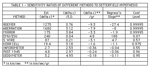
Brown [3] opined that c was constant within the precision of the data. His methodology is seriously flawed [16, p141]. Humphreys [14, p42] questioned why the rate of decrease of c should decrease in direct proportion to our ability to measure it. Humphreys gave no evidence that this was true. As yet no paper has properly addressed this important issue of the sensitivity of the data. First, an estimate of the size of the change in c must be estimated for each method over the interval of time of the different methods used. The quadratic function of Hasofer [13] was used to estimate the difference in values of c at the end points of the various methods and is labeled [Est. (delta) c] in Table 1. The ratio of this estimate to the standard deviation of the method ,which I will call the sensitivity ratio, should be normally distributed. Methods with ratios above 1.65 should be very sensitive to the hypothesized decrease, that is, there is less than a 5% likelihood that the estimated decrease would result from randomness.

The figures in Table 1 represent the sensitivity ratios for methods with 4 or more data as well as the post 1945. These are listed in order of estimated slope(delta c/yr). The EMU/ESU method has been included in the sensitivity analysis for comparison purposes. The statistic was successful in predicting the significance/insignificance of a simple linear regression line in 7 of 9 cases. Five of the six sensitive methods had simple regression line slopes which were significant at the 95% confidence level. Two of the three insensitive methods had insignificant regression lines. If the data with the two smallest ratios(insensitive data) are removed the magnitude of the slopes of their respective regression lines are decreasing significantly and in almost the same order as predicted.

The sensitivity ratio for standing wire values, [21], shows that the standing wire data has insufficient accuracy to distinguish between an empirical trend and randomness. All but the Mercier (1923) datum have been omitted as Birge, Dorsey and Setterfield all included it. The sensitivity of the Roemer data is understated due to the lack of intermediate data. This leads to an artificially high standard deviation. Extra regression lines with and without the Roemer data have been conducted for Table 2. On the other hand the decision to delete all but one of the EMU/ESU data would seem to be well justified by these results. Not only are the data insensitive to the hypothesized change but the direction and magnitude of the slope overall are anomalous.

REGRESSION MODELS

Regression line models are based on three assumptions:

(1) The expected value of the residuals is zero i.e. E[e(i)] = 0

(2) The variance of the errors(residuals) is constant

(3) The errors(residuals) are independent of the random variable

For a regression line to be accepted as a model (not necessarily a unique model) the residuals must be tested for these three conditions. The c data, however, does not easily lend itself to regression analysis. A simple linear regression will not take into account the varying degrees of reliability of the data. A weighted regression technique exists which weights each data with the inverse square of the error bar. This may satisfy condition 2 (homoscedasticity) but for the c data a poor fit. More importantly, this weighting procedure in the case of the c data causes a correlation between the residuals violating condition 3. The residuals are said to be autocorrelated. The standard test for autocorrelation is called the Durban-Watson test. In the case of the c data the autocorrelation stems from the time dependence of the error bars themselves. The standard technique for correction of autocorrelation is to apply an autocorrelation parameter [18,p356] to the data to smooth it prior to regression. Unfortunately, when applied to the weighted regression line for c data the residuals still fail the Durban-Watson test. Even repeated applications are ineffectual at correcting the problem.

To solve this dilemma, a different weighted regression technique will be used. Let T be the independent random variable representing time and C be the dependent random variable representing the velocity of light. The following presents a quadratic regression model:

C(i) = a + bT(i) + dT(i) (exp 2) + e(i) 	 (1)

where a, b, d are coefficients C and T are random variables and e(i), is the error.

If the variance of e, is proportional to T (exp 2), where T is measured in years prior, the variance of e/T is constant and a regression line will be homoscedastic.

[sigma (e) (exp 2)] = k [T (exp 2)]	(2)

where [sigma (e) (exp 2)] is the statistical symbol for variance

Equation (1) is then transformed into

C(i)/T; = a/T(i) + b + DT(i); + e(i)/T(i)		(3)

The variance of the errors is

[sigma (exp 2)] [e(i)/T(i)) = [sigma (exp 2)] [e(i)]/[T(i) exp 2)] 

= k [T(i) (exp 2)]/ [T(i)) (exp 2)] = k		(4)

i.e. the variance of the errors is constant.

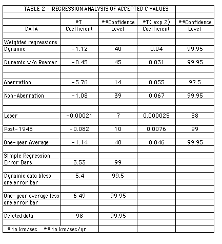
Results of this regression of the data (DAFA) are recorded in Table 2. Dynamic data in the table refers to the whole set of data less the laser data which was timed using atomic rather than dynamic time. The null hypothesis is that there is no decrease in c versus the alternate hypothesis that there is. All 6 tests on the dynamic data and its major subsets showed a significant quadratic term at the 97.5% confidence level. Only the Laser values had insignificant coefficients for both the linear and the quadratic. Note that the time is calculated in years prior to 1967.5 and so positive terms mean an increase in c as one goes back in time. Other methods were also tested. In all cases at least one coefficient is significant and positive. Most of these data sets are too small for their results to be very credible in themselves. However, they are consistent with results of the larger data sets. Kerr cell, standing wire and geodimeter values also had a negative significant value.

Bias

By historical accident some decades and years have more data. This is an historical bias and could led to exaggerated results. To test what bias this influence has a weighted regression was done on the data (DAFA) where values in the same year were replaced by their weighted average. This is listed under One-year Average. The significance level rose indicating this bias lowers the significance of the regression. Simple regressions were also performed on the values less their error bars, i.e. the minimum of their probable values. Since the less reliable data has larger error bars this technique lowers the value of the less reliable data more than the better data. The regression line was still positively and significantly sloped. This was still true at 1.92 times the error bar and the slope was still positive even at 2.47 times the error bar. This should not be true of a set of values representing a constant. Lastly, a simple regression was done on the deleted data. Its slope was decreasing at 98+17 km/sec/yr.

Although significant quadratic relationship has been found in the accepted data and its major subsets, it cannot be assumed that this relationship is due to a physical decrease in the value of c. It has been established that this decrease is empirical and not random.

Other possibilities must be explored as well as the physical one:

(1) Is the decrease dependent on the less reliable 18th century data?

(2) Is the decrease a product of combining methods with systematic or other errors?

(3) Is the decrease a one-sided approach to the current value of c due to experimental or experimenter bias?

To determine the answer to the first question the 18th century values were subtracted from the accepted (DAFA) data. A weighted regression was performed on the remainder. which resulted in a coefficient of T2 significant at the 97 .5 % confidence level. The t test was applied to the average and was significant at the 99.9% confidence level. The removal of the 18th century data does not result in insignificant tests. Could some other data in a specific time interval be responsible for the decrease in the data. Initially a 10 year interval was chosen for analysis but too many of the cells had too little data. The interval was widened to 20 years. Even so, the 18th century data had to be grouped into a single cell and the 1940 cell was moved to 1947-67 to include the 3 extra data.

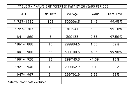
The t tests for the averages of this group of cells is presented in Table 3. Laser results have been omitted. Of the 7 cells 4 have significant deviations from the accepted value of 299792.458 km/sec. This is much higher than would be expected on the basis of random chance. There were no results in the 25-75 percentile range where half the results would be expected to be. The one cell with the obviously anomalous results is the 1900-1920 era where the predominant values are by the aberration method. This suggests that the aberration values are systematically low. The distribution of aberration and nonaberration values about the accepted value was tabulated. Table 4 shows the number of values above and below the accepted value accumulated by 200 km/sec intervals and a binomial statistic and confidence level for each pair.

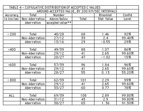
** Accepted value = 299792.458 km/sec

For the non-aberration values the binomial test shows significance at the 99% confidence level throughout all ranges of accuracy. The aberration values on the other hand range from 15% to 91%. Not one of the distributions are significant at the 95% confidence level. Yet from Table 2 regression results both of these subsets yield similar and significant T2 coefficients. In addition, the number of aberration values above the accepted value prior to 1900 is 27 of 35 values whereas the after 1900 the distribution is reversed and there are only 11 of 30. The aberration values as a whole have an insignificant distribution over all ranges of accuracy but is composed of two highly different distributions pre and post 1900. It would be expected that the experimental values ought to approach the accepted value whether from above, below or both. This is true of the non-aberration values but not of the aberration values. From the above considerations it may be concluded that the aberration values are the anomalous ones, that they are decreasing at about the same rate and that they decrease to a value lower than the non-aberration values, i.e. they are systematically low. From the significance of the weighted regressions and the t-test on the post 18th century data it may be concluded that there is still a significant decrease in the values of that era and this despite the effects of a systematic error in the aberration values which reduces the value of the T2 coefficient of the whole data below those of the corresponding aberration and non-aberration values.

The second possible explanation for the decrease in c values is that it is a product of different systematic errors in the various methods. In such cases a significant portion of the methods ought to show constancy. From the results of Table 1 it can be seen that only the EMU/ESU shows a positive slope by simple regression and of those methods which have data sensitive enough to find a decrease all but one have significant slopes. The weighted regression lines show no substantial difference. The aberration and non-aberration coefficients are both significant. The combination of these two in fact decreases the regression coefficients likely because of the systematic error in the aberration values. The omission of the Roemer data still leaves a significant weighted regression line. The post-1945 data is also significant. This leaves 15 other values representing mainly the Kerr cell and optical values. The Kerr cell values are also decreasing with time but because they are all less than the accepted value they actually decrease the size of the slope of the weighted regression model. The optical measurements have a significant linear decrease and an insignificant quadratic coefficient. There is no sign that a set of constant method(s) is(are) causing c values to be misinterpreted as a decreasing trend. In fact, certain systematic problems can be shown to be lowering the rate of decrease in the regression model.

The third possibility is harder to determine since the behavior of the data under the assumption of a physically decreasing value of c and a decreasing value of c due to a one-sided approach to the accepted value is almost the same. The c values do contain at least one example of this kind of phenomenon. The EMU/ESU has a very steep trend in the 1868-1883 range (10 of 25 data) which is 5 times steeper than for the whole data set. The t-test on the average of these two subsets have substantially different confidence levels (99.5% and 40%). As the experiments became more accurate a one-sided negative systematic error was obviously reduced more than all the others. After a certain point the reduction in this error was no longer significant and the values stabilized. This kind of behavior ought to be detectable by arranging the data by error bar size and examining the results for obvious breaks in the significance.

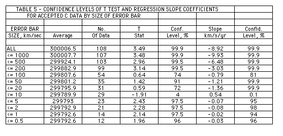
In Table 5, the averages and simple regression slopes for different error bars intervals are listed together with the significance of the their t-tests. If the hypothesis is that the values of c are approaching from one-side due to experimental or experimenter bias than there ought to be a break in the confidence levels. There is such a break at 100 km/sec where significance drops to 74% . However, at 5 km/sec this significance reappears and the confidence levels remains significant down to the .5 km/sec cell after which there is too little data. Furthermore, the difference in the confidence levels between the 5 and 10 km/sec group is over 93 points! This jump is caused by adding only 6 data to 23. These data contain all 4 Kerr cell values which are all below the accepted value by significant amounts. They also prevent significance in the 20 and 50 km/sec group. The 100 km/sec group contains many of the post 1900 aberration values which are systematically low and it would be anticipated that these would have considerable effect on the 100 km/sec cell. The confidence levels of the simple regression lines show an identical pattern; the only cells to show loss of significance are those affected by Kerr cell and post-1900 aberration. The only example of one-sided errors or biases which have affected the values of c to be found are the EMU/ESU values. Although others [14] have mentioned this phenomenon as an explanation for the decrease in the values of c, they have not given examples.

DISCUSSION

A major focus of this paper is to create a set of c values which is appropriate for analysis with respect to the Setterfield hypothesis. It is appropriate to examine what the inclusion of these deletions would have. The inclusion of EMU/ESU data would definitely have a significant influence on all results except the error bar analysis. This method's lack of accuracy and precision cannot justify its inclusion in this analysis. Those who would include this method will no doubt disagree with the conclusions of this analysis. Both the rejected and the outliers, if added back in would augment the size of the decrease in c. They would also increase the initial averages and slopes in the time and error bar analysis.

To ascertain what bias the deletions have as a whole a simple regression line through the deleted data was done. This yielded a 98+17 km/sec/yr decrease. The average (300157 km/sec) was above that of the DAFA data but not significantly. The regression slope is significant despite the inclusion of the EMU/ESU data. It cannot therefore be claimed that results favoring the Setterfield hypothesis are attributable to the bias in the selection of deleted data.

Regression lines have been published by a number of researchers and have played a key role in the debate [1], [4], [9], [13], [16]. It would then be appropriate to give some account of them. Norman's regression lines although significant are all unweighted as are Brown and Evered's tertiary polynomial. None of these are homoscedastic. Aardsma's and Hasofer's published weighted regression lines which are homoscedastic. Aardsma's is linear and not significant and Hasofer's is quadratic and is significant. However, but both fail the Durban-Watson statistic at the 99% confidence level i.e. the residuals of the lines are autocorrelated. In addition, some error bars in Hasofer's regression analysis have been challenged which would change the significance [10, p83]. Thus, no regression line published to date has met all three conditions for a regression line model. It may be noted in defense of Aardsma's work that he was merely constructing an weighted average rate of change. For this purpose he used the required technique. However, in my opinion he has failed to grasp the complexity and systematic errors of the data and thus the need for a broader and deeper analysis.

Several factors led me to this opinion. First, the weighting of Aardsma's line puts over 90% of the weight on 6 data points in the 1956-1967 era. The average unweighted slope in this era is less than a .03 km/sec/yr decrease. Thus there is a bias in the weights of the data towards the era with the smallest slope. In such cases, one must be wary that one's interpretations are valid beyond the small number of data which effectively determine the results. The bias can be lessened by reducing the weighting factor or reducing the number of data where the heaviest weighting occurs. The weighted one-year-average regression line in Table 2 is one such technique. Another possibility would be to regress the pre-1945 data to test whether insignificant change is restricted to the post-1945 data.

Second, the Durban-Watson test for Aardsma's regression line is significant at the 99% confidence level indicating that the residuals from this line still form a significant time dependent sequence: that is, not all the decrease in the data is reflected in the regression coefficient. Furthermore, there are major corrections which must be made to Aardsma's data. Although not stated in Setterfield's paper the EMU/ESU, standing wire and aberration methods contain 92 data for which the in vacuo adjustment has not been made. In addition, several values are duplicates and triplicates which add to the bias. These biases act together to minimize the slope and the significance of his result. Thus, his conclusions are not based on satisfactory evidence.

PREDICTIONS

The quality of a scientific hypothesis must be judged not only by its fit to empirical data but also by its predictions. The effect that a decreasing c would have on other physical constants if the frequency of light were decreasing has been presented by Norman and Setterfield [19}. They claim their analysis verifies the predictions of their hypothesis. Testing of this claim will be the subject of future research. However, there is the question whether Setterfield's distinction between atomic time and dynamic or gravitational time has long term physical effects rather than a minor temporary one. There needs to be a demonstration that over long periods the discrepancy between atomic time and gravitational time is significant. Fortunately, examples can be found.

Stars ages are calculated using atomic isotope ratios of hydrogen and helium. These ratios are interpreted as yielding ages up to billions of years. These ages are in atomic years. However, remnants of supernova stars can dated by various techniques which are dependent on its rate of expansion, a dynamic process. Their ages, according to Davies' [5] analysis of supernova remnants in our galaxy, range up to 7,000-8,000 years in gravitational time. Although age estimations are still crude it must be admitted that a wide discrepancy exists between the atomic ages of stars and gravitational age of supernova remnants and that this is not expected according to conventional theories.

Zircon crystals embedded in deep granites in the Earth's crust and studied by Gentry are dated by Uranium/Lead isotopes ratios (atomic process) to be over a billion years old. However, the rate of diffusion (dynamic process) of the helium byproduct shows the radioactive decay to be 10,000 years old or less [12, p52-53]. Gentry accounts for this age discrepancy by suggesting a supernatural increase in radioactivity during brief periods prior to or during the flood. Whatever the cause, the data cannot be anticipated by the conventional view that atomic and gravitational ages are equivalent. Setterfield's hypothesis predicts what conventional scientists are forced to discount.

Another problem concerns the spiral appearance of many of the galaxies in the universe. In order for spiral galaxies to retain their shape the velocities of the stars within the arms of the spirals ought to vary in direct proportion to their radii. This is not observed. All the stars in the arms within each spiral galaxy have the approximately the same speed [20]. Thus, the stars in the outer portion of the arms, having a much longer orbit, trail farther and farther behind the inner ones as time goes on. Conversely, if one goes back in time the stars on the inner portion of the spirals would back up faster than those in the outer portion and the spiral shape would look less curved. As the astronomers look farther into space they are looking at images of galaxies whose light was emitted earlier in time which ought to appear progressively less curved or less wound-up spiral galaxies. Since the average rotation period is in the order of 200 million years there ought to be some discernible differences beyond 200 million light years. Astronomers have failed to find any such progression in their observations up to l billion light-years [8]. This, too, is a natural consequence of the decreasing c hypothesis in that light travel time is much lower than conventionally assumed because of the higher velocity of light in the past.

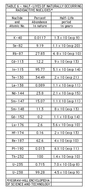
Finally, every radioactive isotope known with an atomic number less than or equal to 92 and a half-life greater than 700 million years is found naturally in the Earth's crust. With the exception of carbon-14 which is produced continually in the upper atmosphere and isotopes which are by-products of other long half-life isotopes there are no short half-life isotopes (less than 700 million years) occurring naturally in the crust [15]. If radioactive decay values were constant and the Earth were 4-5 billion years old then long half-life isotopes should still exist after 4-5 billion years but not the short half-life ones (see Table 6). This evidences agrees with the standard evolutionary geology. Setterfield's hypothesis predicts the same results as the evolutionary model but provides an alternative naturalistic explanation for this distribution, one within a short Earth history. Creationist explanations have focused heavily on individual ratios and methods. I could find no creationist papers which explain the above distribution.

CONCLUSIONS

The above analysis has accepted the published values, reworkings and corrections as valid. This does not mean that new information has not or will not arise to change the assessment of the proper value which should be assigned to the observations. It would be entirely appropriate to reevaluate the published values in light of any new techniques or knowledge. This I leave to the physicists. My purpose here is to provide motivation and justification for such research.

From my analysis it may be reasonably concluded that:

(1) EMU/ESU and standing wire data are too insensitive to test Setterfield's hypothesis.

(2) Both Aberration and Kerr Cell results have systematically low values.

(3) c(t) = 299792 + .031 x [(1967.5-t)(exp 2)] is a suitable regression model for the velocity of light values in the last 250 years.

(4) Tests of the selected data strongly support an decrease in the values of c. No evidence of experimental causes could be found for the observed decrease.

(5) Predictive abilities of the Setterfield hypothesis make a physical interpretation of the empirical decrease not only reasonable but credible.

The regression model in this paper ought to be given priority over previously published regression lines since it is the only one which is weighted, homoscedastic and non-autocorrelated. In addition it is the only one based on one in vacuo datum per experiment. It provides the soundest grounds so far to decide the question. The various non-random distributions of the data by date, precision, accuracy, and method are too consistent and pervasive to have been caused by systematic experimental and experimenter biases. Those biases and systematic errors in the data which can be identified are not helpful in providing a non-physical explanation of the results. The prediction of a substantially divergent ages for dynamic processes proceeding from nuclear processes is a very critical test of the Setterfield hypothesis. There exist physical examples which extend past the three hundred years of data used here. These data are compatible with Setterfield's hypothesis but unexpected from conventional physics. The agreement of statistical and physical evidences provide ample grounds for pursuing physical mechanisms to explain the decrease in the velocity of light.

ACKNOWLEDGMENTS

I am grateful to all those who contribute their time and talents to these conferences. Their energy and commitment are admired. I would also thank Dr. Tom Goss whose professional skills in statistical analysis were not only helpful but were given freely and lovingly despite his busy schedule. Lastly, I would like to thank Lambert Dolphin for his encouragement through the trials of life as well as science.

REFERENCES

[1] G. Aardsma, Has the Speed of Light Decayed Recently? Paper 1, Creation Research Society Quarterly, Vol. 25: 1 (1988) 36-40.

[2] R.T. Birge, The General Physical Constants: as of August 1941 with Details on the Velocity of Light Only, Reports on Progress in Physics 8 (1941) 90-134.

[3] R.H. Brown, Statistical Analysis of the Atomic Constants, Light and Time, Creation Research Society Quarterly Vol. 25:4 (1988) 91-95.

[4] R.H. Brown, Speed of Light Statistics, Creation Research Society Quarterly Vol. 26:4 (1990) 142-143.

[5] K. Davies, The Distribution of Supernova Remnants in the Galaxy, Proceedings of the Third International Conference on Creationism, K. Walsh et al, editors, Vol. 3 (1994), Creation Science Fellowship, Pittsburgh, PA.

[6] G. DeBray, The Velocity of Light, Nature Vol. 120 (1927) 602-604.

[7] N.E. Dorsey, The Velocity of Light, Transactions of the American Philosophical Society, 34 (1944) 1-110.

[8] A. Dressler, Galaxies Long Ago and Far Away, Sky and Telescope Vol. 85:4 (1993) 22-25.

[9] M.G. Evered, Computer Analysis of the Historical Values of the Velocity of Light, Creation Ex Nihilo Tech. J. Vol. 5:2 (1991) 94-96.

[10] M.G. Evered, Further Evidence Against the Theory of a Recent Decrease in c, Creation Ex Nihilo Tech. J. Vol. 6:1 (1992) 80-89.

[11] K.D. Froome and L. Essen, The Velocity of Light and Radio Waves, (1969), Academic Press, NY.

[12] R.V. Gentry, Radioactive Halos in a Radiological and Cosmological Perspective, Proceedings of the 63rd Annual Meeting of the Pacific Division. AAAS (1984), 38-63.

[13] A.M. Hasofer, A Regression Analysis of the Historical Light Measurements, Creation Ex Nihilo Tech. J. Vol. 4 (1991) 94-96.

[14] D.R. Humphreys, Has the Speed of Light Decreased Recently? Paper 2, Creation Research Society Quarterly Vol. 25:1 (1988) 40-45. [15] McGraw-Hill Encyclopedia of Science and Technology, Sixth Ed., Vol. 15 107, McGraw-Hill, NY.

[16] A.L. Montgomery, Statistical Analysis of c and Related Atomic Constants, Creation Research Society Quarterly Vol. 26:4 (1990) 138-142.

[17] J.F. Mulligan and D F. McDonald, Some Recent Determinations of the Velocity of Light II, American Journal of Science Vol. 25 (1957)180-192 [18] J. Neter and W. Wasserman, Applied Linear Statistical Models, 1974, Richard D. Irwin, Homewood, IL.

[19] T. Norman and B. Setterfield, The Atomic Constants. Light and Time, 1987, Invited Research Paper for Lambert Dolphin, SRI International, Menlo Park Clara, CA.

[20] V. Rubin, Dark Matter in Spiral Galaxies, Scientific American, Vol. 248:6 (1983), 96-108.

[21] D.P. Todd, Solar Parallax from the Velocity of Light, American Journal of Science, series 3 Vol. 19 (1880): 59-64.

APPENDIX A: All Data Combined. Date Set: Excel File (CDATALL2.xls) or Data Set: HTML (cdatall3.html)

Entered April 29, 1995